2 Literature review
In this chapter we present a brief literature review particularly focused of stem cells in cancer and the different modelling approaches that have been used.
2.1 Introduction
Stem cells are defined as cells that have the ability to perpetuate themselves through self-renewal and to generate mature cells of a particular tissue through differentiation (Reya et al. 2001). Stem cells are fundamental to tissue maintenance and repair; they also play a critical role in cancer development and in determining the outcomes of cancer treatment (Weiss, Komarova, and Rodriguez-Brenes 2017).
2.2 Stem cells in cancer
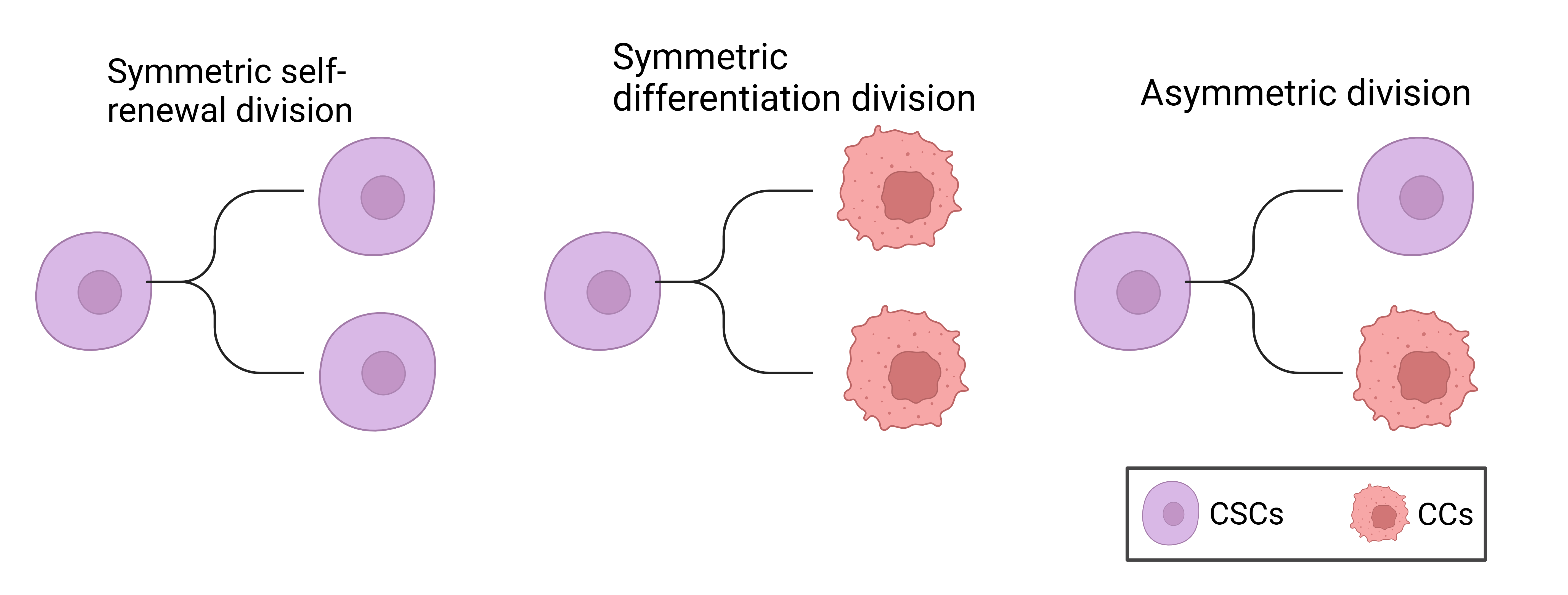
Perhaps the most important and useful property of stem cells is that of self-renewal. Self-renewal is crucial to stem cell function, because it is required by the majority of stem cells to persist for the lifetime of the animal. Moreover, whereas stem cells from different organs may vary in their developmental potential, all stem cells must self-renew and regulate the relative balance between self-renewal and differentiation. Understanding the regulation of normal stem cell self-renewal is also fundamental to understanding the regulation of cancer cell proliferation, because cancer can be considered to be a disease of unregulated self-renewal (Reya et al. 2001). Another distinguishing hallmark of stem cells is the ability to undergo asymmetric division, during which stem cells give rise to daughter cells of different fates, proliferative potential, size or other characteristics (Majumdar and Liu 2020; Hitomi et al. 2021a). Cancer stem cells (CSCs) generate such diverse progeny by executing multiple modes of cell division. Lineage-tracing experiments in glioma stem cells (GSCs) revealed that CSC undergo three main types of cell division: 1) Symmetric CSC self-renewing division, where a CSC produces two daughter CSCs; 2) symmetric differentiating division, where a CSC gives rise to two non-CSC daughter cells; 3) asymmetric division, where a CSC produces one CSC and one non-CSC. Additionally less than 1% of cell divisions resulted in cell death (Lathia et al. 2011). The types of CSC cell division are summarized in Figure 2.1.
Numerous arguments suggest a stem-cell origin for human cancers. First, it is worth noting that stem cells possess many of the features that constitute the tumour phenotype, including self-renewal and essentially unlimited replicative potential (Hanahan and Weinberg 2000). Second, the mutations that initiate tumour formation seem to accumulate in cells that persist throughout a person’s life, as suggested by the exponential increase of cancer incidence with age (Meza et al. 2008). This is thought to reflect a requirement for between four and seven mutations in a single cell (and its progeny) to effect malignant transformation (Hanahan and Weinberg 2000). Similarly, cancer formation from cells that persist throughout life is suggested by an increased incidence in adults of skin tumours such as melanoma after higher childhood exposure to a mutagenic agent such as ultraviolet solar radiation (Balk 2011). Normal somatic stem cells are strong candidates for such persistent cells, an alternative explanation would be that a more mature cell undergoes a dedifferentiation event, reverting to a more primitive stem cell phenotype (Sell 1993; Reya et al. 2001).
A stem cell origin for human cancers was first identified in leukaemia, perhaps due to the high fraction of stem cells in the haematopoietic system, when it was discovered that some, but not all, cancer cells were able to initiate tumours of the blood (Taipale and Beachy 2001; Lapidot et al. 1994; Bonnet and Dick 1997). More recently CSCs have been identified in many solid tumours including breast, colon and brain (Al-Hajj et al. 2003; Ricci-Vitiani et al. 2007; Ignatova et al. 2002; Hemmati et al. 2003; Singh et al. 2004; Galli et al. 2004). In GBM, cells expressing the CD133 cell surface protein marker (also found on neural stem cells) have been identified as having stem cell properties in vitro (Singh et al. 2003). Furthermore, when tested using a xenograft assay, it was found that injection of as few as 100 CD133+ cells produced a tumour that could be serially transplanted and was phenotypically similar to the patient’s original tumour, while injection of \(10^5\) CD133- cells survived in the host but did not cause a tumour (Singh et al. 2004). This provides strong evidence that there is a small subpopulation of glioma stem cells that have the unique ability to initiate tumours, while the majority of cells cannot.
2.3 Cancer stem cells and treatment resistance
Radiation therapy is the most common form of treatment across all cancers, with around 50% of all cancer patients receiving radiotherapy at some point in their treatment (Baskar et al. 2012). However, in addition to being tumour-initiating, CSCs are highly resistant to both radio- and chemo-therapy through preferential activation of the DNA damage checkpoint response and an increase in DNA repair capacity (Bao et al. 2006; Tang et al. 2021a; Rich 2007; Schonberg et al. 2014). In glioma, experimental results have shown that both in culture and mouse models CD133-expressing stem cells survive radiation in larger proportions than the majority of tumour cells which lack CD133 expression (Bao et al. 2006; Gao et al. 2013); these results suggest that CSC confer radio-resistance in GBM and ultimately are the source of tumour recurrence after radiation.
In addition to being resistant to treatment CSCs also engage in a synergistic relationship with the surrounding tumour microenvironment to promote angiogenesis, proliferation, migration, tumour survival, and immune evasion (Ma et al. 2018; Rich 2007). Taken together this highlights the important role CSCs play in determining tumour response to therapy. There is a desperate need for targeted therapies that either directly kill CSCs or sensitize CSCs to standard cytotoxic therapies in order to improve treatment outcomes.
2.4 Mathematical models of cancer stem cell dynamics
Many different mathematical models have been developed to model stem cell dynamics. Understanding CSC kinetics and interaction with their non-stem counterparts is still limited; theoretical and mathematical models may help elucidate their role in cancer progression and treatment response. Here we focus on a subset of models used in the literature that cover a wide range of modelling techniques and have particularly inspired our modelling used in the preprint presented at the end of this report.
Many of the following models use slightly different terminology to refer to the non-stem cell population such as cancer cell, progenitor cells or tumour cells, for clarity we will refer to non-stem cells always as cancer cells (CCs) throughout this review.
2.4.1 Agent-based models
In (Enderling et al. 2009) and (Gao et al. 2013) the authors develop an agent-based model (ABM) to study the dynamics of CSCs and CCs in a tumour. It is assumed that tumours are a heterogenous mix of CSCs and CCs. Cells are considered as individual entities with a cell cycle and limited proliferation capacity \(\rho \in [0,\rho_\text{max}]\). CSCs have unlimited self-renewal, hence \(\rho_\text{max} = \infty\). At each cell division CSCs can undergo symmetric self-renewing division with probability \(\delta\) or asymmetric division with probability \(1-\delta\). The proliferation capacity \(\rho\) is decremented at each CC division and inherited by both daughter cells.
Simulations of the ABM model revealed the following key results:
- Tumours developing solely from CCs will inevitably die out, due to their limited proliferation capacity. Hence, CSCs are necessary for malignant tumour growth. This is consistent with experimental results showing only CSCs can initiate tumours (Lapidot et al. 1994; Singh et al. 2004).
- Tumours started from a single CC could still persist for a long time as long-term dormant lesions, but due to space-limited growth remain small – well below the potential maximum size of \(2^{\rho_\text{max}}\). Significant growth only occurs once a CSC is initiated. In fact, even with a single CSC, the tumour may remain small for an extended period due to space-limited growth. This is consistent with the observation that many tumours remain dormant for many years before they start to grow (Sweeney 1995; Neves-E-Castro 2006; Folkman and Kalluri 2004).
- A high rate of spontaneous death of CCs actually enables room for sufficient stem cell divisions to enrich the stem cell pool and drive tumour growth. This leads to what they call the “tumour growth paradox”, where counterintuitively an increase in the death rate of CCs decreases the total tumour size in the short term, in the long run it leads to an increase in the total tumour size as the tumour contains more CSCs.
Mathematically the tumour growth paradox is defined as follows.
Definition 2.1 (Tumour growth paradox) Let \(N_\alpha (t)\) denote a total tumour population with death rate \(\alpha\) for CCs. The population exhibits a tumour growth paradox if there exist death rates \(\alpha_1 < \alpha_2\) and times \(t_1,t_2, T\) and \(T_0\) such that
\[ \begin{aligned} N_{\alpha_1}(t_1) = N_{\alpha_2}(t_2)& \quad \text{and} \quad N_{\alpha_1}(t_1 + T) < N_{\alpha_2}(t_2 + T) \\ &\text{for} \quad (0<T<T_0), \end{aligned} \tag{2.1}\]
2.4.2 Integro-differential model
Following on from the ABM developed in (Enderling et al. 2009; Gao et al. 2013), in (Hillen, Enderling, and Hahnfeldt 2013) the authors develop an integro-differential equation version of the model, based on the same assumptions as in (Enderling et al. 2009; Gao et al. 2013) outlined in Section 2.4.1. Let \(u(x,t)\) denote the density, in cells per unit space, and let \(v(x,t)\) denote the density of CCs. Hence, the total tumour density is denoted \(N(x,t) = u(x,t) + v(x,t)\). For this analysis cells are assumed to be very small compared to the size of the tissue domain \(\Omega\) (which we take without loss of generality to have unit volume). It is also assumed that cells cannot pile on top of each other so there is a maximum density of one cell per unit space, this implies \(N(x,t) \leq 1\). Cells can only proliferate if there is space to place the daughter cells, otherwise reproduction is inhibited (cellular quiescence). To model the spatial search for space, they define a nonlinear integral term, consistent with the ABM (Enderling et al. 2009; Gao et al. 2013) they assume that all cells can migrate randomly, which is modelled by simple diffusion. These assumptions lead to the following system of equations to describe CSC and CC dynamics:
\[ \begin{aligned} \underbrace{\frac{\partial u(x,t)}{\partial t}}_\text{Rate of change CSCs} &= \underbrace{D_u \nabla^2 u}_\text{Diffusion of CSCs} + \underbrace{\delta \gamma \int_{\Omega} k(x,y,N(x,t))u(y,t) dy}_\text{Self-renewal of CSCs} \\ \underbrace{\frac{\partial v(x,t)}{\partial t}}_\text{Rate of change CCs} &= \underbrace{D_v \nabla^2 v}_\text{Diffusion of CCs} + \underbrace{(1-\delta) \gamma \int_{\Omega} k(x,y,N(x,t))u(y,t) dy}_\text{Differentiation of CSCs} + \\ & \underbrace{\rho \int_{\Omega} k(x,y,N(x,t))v(y,t) dy}_\text{Proliferation of CCs} - \underbrace{\alpha v}_\text{Apoptosis of CCs}. \end{aligned} \tag{2.2}\]
The spatial distribution kernel \(k(x,y,N)\) describes the rate of progeny contribution to location x for a cell at location y per “cell cycle time” i.e., the defined period between divisions of a freely cycling cell. Since greater density at \(x\) would be expected to hinder progeny occupation it is assumed that \(k\) is monotonically decreasing in \(N\), with \(k(x,y,N(x,t))=0\) at \(N=1\). The number of cell cycle times per unit time of CSCs and CCs are denoted by \(\gamma\) and \(\rho\), respectively, and for simplicity it is assumed that \(\gamma = \rho = 1\) throughout. The parameter \(\delta\) with \(0 \leq \delta \leq 1\), as in the ABM (Enderling et al. 2009; Gao et al. 2013), denotes the fraction of CSC divisions that are symmetric self-renewal, while \(1-\delta\) is the fraction of asymmetric divisions. The parameter \(\alpha\) denotes the spontaneous death rate of CCs. Background cell motility is modelled by the diffusion coefficients \(D_u\) and \(D_v\) for CSCs and CCs, respectively. The system is considered to hold in a smooth bounded domain \(\Omega\), with homogeneous Neumann or Dirichlet boundary conditions.
Homogeneous Neumann boundary conditions correspond to a boundary that is impenetrable by cells, this could for example represent a tissue surrounded by membranes, smooth muscle tissue, or bone, and are given by
\[ \frac{\partial u}{\partial n} = 0, \quad \frac{\partial v}{\partial n} = 0 \quad \text{on} \quad \partial \Omega, \tag{2.3}\]
where \(\partial / \partial n\) is the normal derivative at the boundary. The redistribution kernel can only redistribute cells within this domain \(\Omega\), hence we impose
\[ k(x,y,N) = 0 \quad \text{for} \quad x \notin \Omega. \tag{2.4}\]
Homogeneous Dirichlet boundary conditions correspond to a boundary that cells can freely leave but not re-enter again, for example this could represent intravasation into adjacent blood vessels, and are given by
\[ u = 0, \quad v = 0 \quad \text{on} \quad \partial \Omega. \tag{2.5}\]
The redistribution kernel describes transport of cells out of the domain but does not allow entering from the outside in, hence
\[ k(x,y,N) = 0 \quad \text{for} \quad y \notin \Omega. \tag{2.6}\]
Based on these two boundary conditions we can model any combination of domains such as partially covered by membranes, partially permeable membranes and adjacent blood vessels.
2.4.3 ODE model reduction
In order to analyse this model analytically (Hillen, Enderling, and Hahnfeldt 2013) reduce the system of integro-differential equations (Equation 2.2) to a system of ordinary differential equations in the following way.
Reduction 1: Progeny placement depends only on the density at the destination
In this case \(k(x,y,N(x,t)) = k(N(x,t))\). Introducing mean densities which, given that the domain \(\Omega\) has unit volume, can be written as
\[ \bar{u}(t) = \int_{\Omega} u(y,t) dy, \quad \bar{v}(t) = \int_{\Omega} v(y,t) dy, \quad \bar{N}(t) = \bar{u}(t) + \bar{v}(t). \tag{2.7}\]
Then Equation 2.2 becomes:
\[ \begin{aligned} u_t(x,t) &= D_u \nabla^2 u(x,t) + \delta k(N(x,t))\bar{u}(t), \\ v_t(x,t) &= D_v \nabla^2 v(x,t) + (1-\delta) k(N(x,t))\bar{u}(t) + k(N(x,t))\bar{v}(t) - \alpha v(x,t). \end{aligned} \tag{2.8}\]
Reduction 2: Density is uniform across the domain
If tumour growth is assumed uniform across the domain then, \(k(N(x,t)) = k(\bar{N}(t))\) and \(u(x,t)\) and \(v(x,t)\) can be replaced with their spatially averaged values (\(\bar{u}(t)\) and \(\bar{v}(t)\)) and diffusion is zero everywhere. Therefore, Equation 2.8 becomes:
\[ \begin{aligned} \frac{d \bar{u}}{dt} &= \delta k(\bar{N}(t)) \bar{u}, \\ \frac{d \bar{v}}{dt} &= (1-\delta) k(\bar{N}(t)) \bar{u} + k(\bar{N}(t)) \bar{v} - \alpha \bar{v}(t), \end{aligned} \tag{2.9}\]
where the volume filling constraint \(k(\bar{N})\) is taken to be
\[ k(\bar{N}) = \text{max} \left\{0, 1 - \bar{N}^\sigma \right\}, \quad \text{for} \quad \sigma > 1. \tag{2.10}\]
An exponent of \(\sigma = 1\) corresponds to a linearly decreasing rate of occupancy for newborn cells as the total density \(\bar{N}\) increases. Since cells are nonrigid, deformable and able to squeeze into available spaces (Hillen, Enderling, and Hahnfeldt 2013) argue that \(\sigma > 1\) is appropriate and take it to be \(\sigma = 4\), in all their simulations.
Without a CSC population \(\bar{u}(t)\), the density of CCs \(\bar{v}(t)\) satisfies the equation
\[ \frac{d\bar{v}}{dt} =K(\bar{v}(t))\bar{v}(t) - \alpha \bar{v}(t). \tag{2.11}\]
Since \(K(\bar{v}(t))\) is a decreasing function of \(\bar{v}(t)\) the CC population will die out when \(\alpha > k(0)\). Note that this does not specifically set a limited proliferation capacity for CCs, as was the case in (Enderling et al. 2009), rather if \(\alpha > k(0)\) then \(\alpha > k(N)\) for all \(N\) hence the CC population will never survive on its own.
This simpler ODE model allows for analysis of the steady states, from which it can be shown that the pure stem cell steady state \((u,v)= (1,0)\) is a global attractor. Therefore, this model predicts that for long times the tumour will consist of only stem cells. Intermediate tumour composition and the time at which the steady state is achieved are dependent on cell death rate \(\alpha\). The convergence to \((1,0)\) is somewhat surprising as typically the CSC compartment is considered small, comprising only 1-3% of the total tumour (Bao et al. 2006). This suggests that the model may miss key biological dynamics of the CSCs such as some stem cell death and feedback regulation of symmetric / asymmetric division. However, (Hillen, Enderling, and Hahnfeldt 2013) argue that this does not interfere with their analysis, as they are interested in the intermediate time dynamics of tumour initiation and growth, rather than the long-term behaviour as \(t \rightarrow \infty\).
2.4.4 Stochastic model of CSC dynamics
In (Turner et al. 2009), the authors develop a stochastic model for the dynamics of CSCs and CCs, particularly for the case of brain cancer. This stochastic model is particularly appropriate for situations in which small numbers of cells are present such as in vitro or in the early stages of tumour formation. In these cases stochastic fluctuations may have significant effects and cannot be neglected. To study larger populations the authors then derive a deterministic ODE model, based on the stochastic master equation, that describes the average number of CSCs and CCs.
The model assumptions on CSCs and CCs are largely similar as those given previously in Section 2.4.1. However, one key difference is that CSCs are assumed not to be immortal so have some probability of death. Defining \(p(n_s, n_p,t)\) as the probability that there are exactly \(n_s\) CSCs and \(n_p\) CCs at time \(t\), the stochastic master equation is given by
\[ \begin{aligned} \frac{dp(n_s,n_p,t)}{dt} = & \ \rho_s \left[ \underbrace{r_1 (n_s - 1) p(n_s - 1, n_p, t)}_{\text{symmetric self renewal of CSCs}} \right. \\ & + \underbrace{r_2 n_s p(n_s, n_p - 1, t)}_{\text{asymmetric division of CSCs}} \\ & + \underbrace{r_3 (n_s + 1) p(n_s + 1, n_p - 2, t)}_{\text{symmetric differentiation of CSCs}} \\ & \left. - \underbrace{n_s p(n_s, n_p, t)}_\text{Overall division} \right] \\ & + \underbrace{\Gamma_s \left[ (n_s + 1) p(n_s + 1, n_p, t) - n_s p(n_s, n_p, t) \right]}_\text{Apoptosis of CSCs} \\ & + \underbrace{\Gamma_p \left[ (n_p + 1) p(n_s, n_p + 1, t) - n_p p(n_s, n_p, t) \right]}_\text{Apoptosis of CCs}. \end{aligned} \tag{2.12}\]
This model explicitly accounts for all three types of CSC division shown in Figure 2.1 where \(r_1=\) symmetric self renewal probability, \(r_2=\) asymmetric division probability, \(r_3=\) symmetric differentiation probability, and \(\rho_s\) represents the overall CSC division rate. While the model in Section 2.4.2 only accounts for asymmetric division it can be shown that these two formulations are equivalent for a large set of parameter values (Hillen, Enderling, and Hahnfeldt 2013). The parameters \(\Gamma_s\) and \(\Gamma_p\) represent the rate of apoptosis for CSCs and CCs respectively. Due to the model’s stochastic nature, and the inclusion of a death probability for CSCs, it can be shown that the occurrence of a single CSC will not necessarily result in a tumour, even if the probability of self-renewal is greater than the probability of differentiation. This is in contrast to the previous models discussed (Enderling et al. 2009; Hillen, Enderling, and Hahnfeldt 2013) and to a deterministic version of this model (Equation 2.13) that would predict exponential growth of the tumour from a single CSC.
For larger cellular populations it becomes more challenging to simulate such a stochastic model and it becomes pertinent to consider the equations for the average number of CSCs and CCs. Defining the mean cellular populations \(S = <n_s>\), \(P = <n_p>\) and \(r = r_1 - r_3\) (i.e., the difference in symmetric self-renewal division and asymmetric differentiation division), the deterministic model is given by
\[ \begin{aligned} \frac{dS}{dt} &= \rho_s r S - \Gamma_s S, \\ \frac{dP}{dt} &= \rho_s (1-r) S - \Gamma_p P. \end{aligned} \tag{2.13}\]
This model is largely similar to the ODE model presented in (Hillen, Enderling, and Hahnfeldt 2013), Equation 2.9. The main differences are that Equation 2.13 includes a rate of CSC apoptosis \(\Gamma_s\) and Equation 2.13 does not account for completion for space. Although (Turner et al. 2009) introduce this into a later version of the model, where they take \(\rho_s\) to be given by \(\rho_s(S,P) = \rho_s(1 - c_s S - c_p P)\), where \(1/c_s\) and \(1/c_p\) are the limiting populations of stem and CCs respectively. However, a limitation of this approach is that it does not account for competition between CSCs and CCs for space and resources.
2.4.5 A multispecies PDE model of cell lineages
In (Youssefpour et al. 2012) the authors develop a multispecies PDE model for CSC lineage dynamics. This is the first model we have looked at that considers more than the two cell types, CSCs and CCs. Here the model is more complex and accounts for CSCs, committed progenitor cells, terminal cells, and dead cells. As with the previous models we have looked at it is assumes that differentiation and feedback processes link the cells’ lineage through self-renewal fractions and mitosis rates. The dependent variables in the model are the local volume fractions of the cell species denoted \(\phi_\text{CSC}, \phi_\text{CP}, \phi_\text{TC}, \phi_\text{DC}\), as well as healthy cells and water \(\phi_\text{H}, \phi_\text{W}\). Assuming there are no voids the sum of the volume fractions equals 1 and each cell type follows a conservation equation of the form
\[ \frac{\partial \phi}{\partial t} = - \nabla \cdot J - \nabla \cdot (u_s \phi) + S \tag{2.14}\]
where \(\phi\) denotes the volume fraction of the cell type, \(J\) is generalized diffusion, \(u_s\) is the mass-averaged velocity of the solid components, \(S\) denotes the mass-exchange terms. This type of multiphase volume fraction approach has been widely used in cancer modelling (Lowengrub et al. 2010; Breward 2003; Hubbard and Byrne 2013). Simulation of this model show that the distributions of cell populations obtained from ABM model (Enderling et al. 2009) and if this mutlspecies model are different. In the ABM CSCs tend to be located either at the center of small tumour clusters or distributed relatively uniformly throughout the tumour, some CSCs may migrate past the tumour boundary and generate new tumour clusters that eventually join the primary cluster crating an irregular boundary. On the other hand, the continuum model finds that CSCs tend to be located at the boundary of sufficient large tumour spheroids, this is consistent with some experiments (Vlashi et al. 2009). For smaller spheroids the CSCs may be more uniformly distributed. The patterns of CSCs and CCs are due to the cell signaling model implemented, detailed in Section 2.5.1, where the CSC self-renewal fraction is regulated by feedback factors produced by the different cells types (Youssefpour et al. 2012).
2.5 Models of differentiation therapy
If, as with normal tissues, cellular phenotypic heterogeneity within tumours can be explained by a hierarchy of differentiation, with only a subset of stem-like cells capable of long-term self-renewal, this raises the prospect that signals promoting differentiation could be effective at driving malignant cells to a less aggressive and ideally post-mitotic differentiated state (Carén, Beck, and Pollard 2016). This differentiation therapy approach has seen success in acute promyelocytic leukemia (APL) where all-trans-retinoic acid (ATRA) can promote differentiation of CSCs and lead to complete remission (Yan and Liu 2016; De Thé 2018). In GBM, bone morphogenetic protein 4 (BMP4), a member of the TGF-\(\beta\) superfamily, has shown potential as a differentiation therapeutic agent. BMP4 has been shown to drive differentiation of GSCs towards a predominantly glial (astrocytic) fate, to reduce GBM tumour burden in vivo and to improve survival in a mouse model of GBM (Nayak et al. 2020; Piccirillo et al. 2006). Despite its potential as a treatment option relatively few mathematical models have considered its possible effects on tumour growth (Youssefpour et al. 2012; Bachman and Hillen 2013; Turner et al. 2009).
2.5.1 Differentiation promoter and self-renewal promoter
In (Youssefpour et al. 2012) they follow (Lander et al. 2009) and assume that the proliferation and differentiation of CSCs are regulated by factors in the tumour microenvironemnt that feedback on self-renewal fractions and mitosis rates. In particular, they denote the differentiation promoter \(T\) (for TGF-beta superfamily members) that reduces the probability of self-renewal for CSCs. They also account for self-renewal promoter \(W\) which increases the probability of self-renewal of CSCs, as well as an inhibitor of \(W\) denoted \(WI\). Possible self-renewal promoters include WNTs, Notch and Shh (Pannuti et al. 2010; Bailey, Singh, and Hollingsworth 2007). Using the notation introduced in Section 2.4.5, they define the CSC self-renewal fraction as
\[ P_s = P_\text{min} + (P_\text{max} - P_\text{min}) \left( \frac{\xi C_w}{1 + \xi C_W} \right)\left( \frac{1}{1 + \psi C_T} \right), \tag{2.15}\]
where \(P_\text{min}\) and \(P_\text{max}\) are the minimum and maximum probability of CSC self-renewal, taken to be \(0.2\) and \(1\) respectively. \(C_W\) and \(C_T\) represent the concentrations of the self-renewal promoter and differentiation promoter respectively. The parameters \(\xi\) and \(\psi\) quantify the sensitivity of CSCs to the regulating proteins.
The concentrations of differentiation promoter and self-renewal promoter are then modelled as follows. It is assumed that \(T\) is more diffuse than either \(W\) or \(WI\). Therefore, on the time scale of cellular proliferation they make the quasi-steady-state assumption that time derivatives and advection of \(T\) can be neglected. Thus, the quasi-steady reaction-diffusion equation for \(C_T\) is given by
\[ 0 = \nabla \cdot (D_T \nabla C_T) - \left( \nu_{UT} \phi + \nu_{DT} \right) C_T + \nu_{PT}\phi_{TC} \tag{2.16}\]
where \(D_T\) is the diffusion coefficient, \(\nu_{UT}\), \(\nu_{DT}\) and \(\nu_\text{PT}\) are the uptake rate by CSCs, the rate of decay and the rate of production by the terminal cells, respectively.
To model the self-renewal promoter \(W\) and its inhibitor \(WI\) a generalized Gierer-Meinhard-Turing system of reaction advection diffusion equations is used, given by
\[ \begin{aligned} &\frac{\partial C_W}{\partial t} + \nabla \cdot (u_s C_W) = \nabla \cdot (D_W \nabla C_W) + f(C_W, C_{WI}), \\ &\frac{\partial C_{WI}}{\partial t} + \nabla \cdot (u_s C_{WI}) = \nabla \cdot (D_{WI} \nabla C_{WI}) + g(C_W, C_{WI}), \end{aligned} \tag{2.17}\]
where
\[ \begin{aligned} f(C_W, C_{WI}) &= \nu_{PW} \frac{C^2_W}{C_{WI}}C_0 \phi_\text{CSC} - \nu_{DW} C_W + u_0C_0 (\phi_\text{CSC} + \phi_\text{CP} + \phi_\text{TC}), \\ g(C_W, C_{WI}) &= \nu_\text{PWI}C^2_W C_0 \phi_\text{CSC} - \nu_\text{DWI} C_{WI}. \end{aligned} \tag{2.18}\]
The parameters \(D_W\) and \(D_{WI}\) are the diffusion coefficients, \(\nu_\text{PW}\), \(\nu_\text{DW}\) and \(\nu_\text{PWI}\), \(\nu_\text{DWI}\) are the production and decay rates of \(W\) and \(WI\) respectively. The parameter \(u_0\) represents a low-level source of \(W\) from all the tumour cells.
To model differentiation therapy (Youssefpour et al. 2012) fix \(\psi = 0.5\) and introduce an external source of \(T\) i.e., a constant source term is added to Equation 2.16.
2.5.2 No self-renewal promoter
In (Bachman and Hillen 2013) they follow (Youssefpour et al. 2012) and model differentiation therapy through a relationship between the average level of differentiation promoter, which they denote \(C_F\) and the probability of CSC self-renewal \(P_s\). However, they do not include the effects of a CSC self-renewal promoting factor, thus
\[ P_s(t) = P_\text{min} + (P_\text{max} - P_\text{min}) \left( \frac{1}{1 + \psi C_F(t)} \right), \tag{2.19}\]
where the notation is the same as in Equation 2.15. Since (Bachman and Hillen 2013) do not model endogenous production of differentiation promoter, \(C_F\) solely represents the level of differentiation promoter prescribed during differentiation therapy. To address this lack of endogenous differentiation promoters they take \(P_\text{max} = 0.505\) (which is equivalent to setting \(\delta = 0.01\) as was done in (Hillen, Enderling, and Hahnfeldt 2013)) and \(P_\text{min} = 0.2\), as is done in (Youssefpour et al. 2012).
As (Bachman and Hillen 2013) use the ODE model developed in (Hillen, Enderling, and Hahnfeldt 2013) they must also develop a submodel for the average level of differentiation promoter. As it is an ODE model they consider the average level of differentiation promoter within a spatially homogeous tumour \(C_F(t)\). It is assumed that the tumour resides within a spherical region of tissue and that differentiation promoter enters this area through the boundary. The differentiation promoter enters the region from the boundary and will diffuse very quickly and attain a steady state distribution over this region. To compute the value of \(C_F(t)\) they solve the problem of diffusion over a sphere of radius \(R\) and average the solution over the volume of the sphere. We use the lower case letter to describe the radial symmetric solution \(c_F(r,t)\) of the following boundary value problem
\[ \begin{aligned} \frac{\partial c_F}{\partial t} &= \omega \left( \frac{\partial}{\partial r} \left(\frac{\partial c_F}{\partial r} \right) + \frac{2}{r} \frac{\partial c_f}{\partial r} \right) \\ c_F(R,t) &= C_{F0}(t), \end{aligned} \tag{2.20}\]
where \(\omega\) is the effective diffusivity of the differentiation promoter. Before differentiation therapy begins \(C_{F0}(t) = 0\), when differentiation therapy begins the boundary condition on the sphere is set to \(C_{F0}(t) = 1\), and the promoter diffuses into the sphere. When differentiation therapy ends, the boundary condition is simply set to 0 and the promoter diffuses out of the sphere. They then set
\[ C_F(t) = \frac{3}{R^3} = \int^R_0 c_F (r,t) r^2 dr. \tag{2.21}\]
2.5.3 BMP4 in glioma
In the previous models (Youssefpour et al. 2012; Hillen, Enderling, and Hahnfeldt 2013) they considered a general differentiation promoter, in (Turner et al. 2009) they consider the specific differentiation promoter BMP4 in GBM. As in the case for the general differentiation promoter they interpret the effects of BMP4 as decreasing the net symmetric division rate \(r\) (following the notation used in Section 2.4.4). Based on (Piccirillo et al. 2006) they estimate that from a pre-treatment value of \(r = 0.1\) the effect of BMP4 is to reduce \(r\) to \(-0.1\), note that following the notation used in Section 2.4.4 \(r\) is defined as \(r = r_1-r_3\) so a change of \(r\) to negative represents a both an increase in the proportion of symmetric differentiation divisions and a decrease in symmetric self-renewal divisions. To model differentiation therapy the parameter value \(r\) is simply switched between these two values for the duration of BMP4 exposure.
2.5.4 Summary of differentiation therapy results
All the models compare 3 different treatment cases radiation alone, differentiation therapy alone and combination therapy. Importantly, as has been shown, all models assume that CSCs are less sensitive to radiation than CCs (Bao et al. 2006; Tang et al. 2021b; Hitomi et al. 2021b). Despite the slight differences in assumptions and implementation, all models find similar results. Radiotherapy alone fails as some CSCs survive and are able to repopulate the tumour. In fact, all models show an extension of the “tumour growth paradox” which we term the “tumour treatment paradox”. When treating with radiation alone the fraction of CSCs increases, since the CCs are more susceptible they significantly reduce their numbers leaving more room for CSCs. This CSC enriched post-treatment state allows much more rapid re-growth of the tumour. This suggests that current standard of care treatment selects for the more resistant CSCs. Thus treatment often facilitates more rapid and aggressive tumour recurrence. Differentiation therapy alone can successfully eradicate the tumour, however, given all models assume that CSCs can only transform into CCs through cellular division, rather than direct transition, large intermediate values of total tumour size may be reached using this approach. Combination of differentiation and radiotherapy out performed either single therapies, often showing that the tumour can be driven to much smaller sizes and potentially extinction. This is because the differentiation agent induces CSCs to turn into CCs which then can be killed by traditional radiation therapy. This combination therapy can be considered a new class of strategies for cancer therapy known as evolutionary steering approaches. Rather than reactively altering treatment as resistance is acquired we proactively select our treatment to minimise resistance and increase chance of extinction (Enriquez-Navas, Wojtkowiak, and Gatenby 2015; Acar et al. 2020).
2.6 Conclusion
In summary, mathematical models of CSC dynamics provide valuable insights into tumour growth, dormancy, and response to treatment. While the models reviewed here vary in their complexity and underlying assumptions, they all highlight the critical role of CSCs in tumour maintenance, treatment resistance and tumour recurrence. Mathematical modelling provides a unique tool for analysing the non-trivial interaction between CSCs and CCs that can arise from fairly simple assumptions, allowing us to verify or generate new hypothesis in order to better understand the role of CSCs.
The differentiation therapy approach aims to drive CSCs within tumours toward a differentiated state, potentially mitigating their self-renewal capacity and aggressiveness. Despite this, many challenges remain in developing differentiation therapies that can be used in a clinical setting (Carén, Beck, and Pollard 2016). One key challenge particularly in GBM is delivery of differentiation therapy to the tumour microenvironment, due to the blood brain barrier (BBB) which limits transport into the brain. New delivery mechanism to combat this are being developed such as adipose derived mesenchymal stem cells, containing BMP4 in nanoparticles. These can be delivered directly into the tumour at the time of resection or systemically as they have been shown to cross the BBB (Li et al. 2014; Mangraviti et al. 2016; Pendleton et al. 2013). Additionally as with all therapies there is vast heterogeneity between patient response to differentiation therapy, indicating the importance of identifying biomarkers for sensitivity to such therapies. In work in preparation it has been shown that GBM cell lines that did not express pRBS were unresponsive to differentiation therapy (Farias et al., n.d.). Mathematical modelling may also help improve the effectiveness of differentiation therapy strategies optimising its delivery in combination with standard cytotoxic therapies as well as elucidating the mechanism through which CSCs drive tumour growth.
In the next chapter I present our preprint, looking at a model for BMP4 induced differentiation therapy in GBM, which is available on bioR\(\chi\)iv Virtual Clinical Trials of BMP4 Differentiation Therapy: Digital Twins to Aid Glioblastoma Trial Design.